scenarioStochasticDragSpacecraft

This scenario mirrors examples/mujoco/scenarioStochasticDrag.py but uses the spacecraft.Spacecraft dynamics model (spacecraft.h based) together with MeanRevertingNoiseStateEffector.

The atmospheric density used by drag is:

\[\rho_{\text{stoch}} = \rho_{\text{exp}}(1 + \delta_\rho)\]

where \(\delta_\rho\) is an Ornstein-Uhlenbeck process implemented as a state in the state effector.

Alternatively, running with useIgbm=True uses C++ Module: igbmNoiseStateEffector instead: the factor \((1 + \delta_\rho)\) then follows an inhomogeneous geometric Brownian motion (multiplicative noise). Its exact process is positive and mean-reverting, so it is a natural model for a positive density factor; C++ Module: dragDynamicEffector clamps the corrected density to be non-negative to guard against the rare non-positive value an explicit integrator can produce. Both models are configured with the same stationary standard deviation and time constant, so the two runs are statistically comparable.

Illustration of Simulation Results

The following images illustrate a possible simulation result.

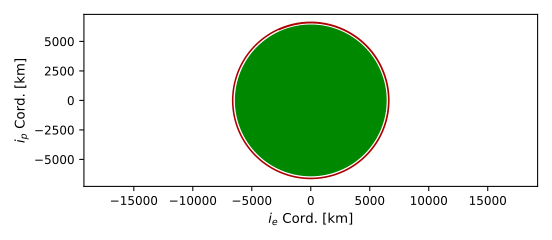
The orbit is plotted in the orbital plane:

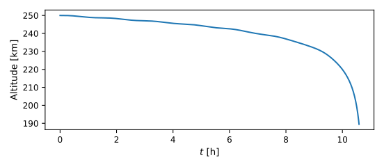
The altitude as a function of time is plotted.

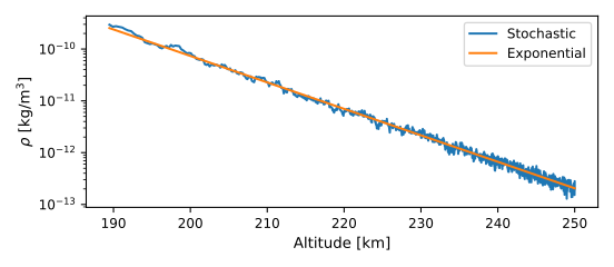
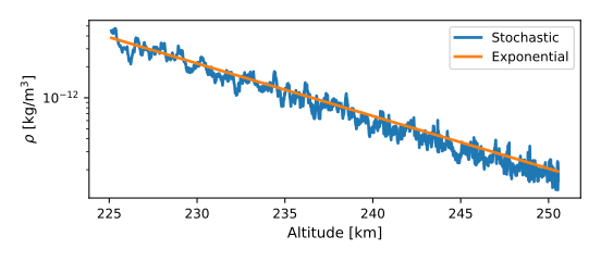
The atmospheric density as a function of altitude is plotted in lin-log space. This shows two lines: the deterministic, exponential density (should appear linear); and the stochastic density.

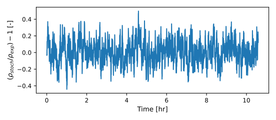
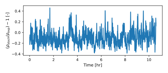
The atmospheric density correction, which should have a standard deviation of 0.15.

The magnitude of drag force over time is plotted in lin-log space.

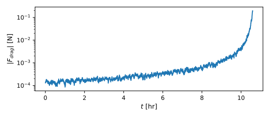
Illustration of Simulation Results with IGBM

The following images illustrate a possible simulation result with useIgbm=True (figure names gain an igbm tag). The overall trajectory is statistically similar to the OU case since both processes share the same stationary standard deviation and time constant; the qualitative difference is in the density factor, which is a positive mean-reverting multiplicative factor under IGBM.

The atmospheric density as a function of altitude:

The atmospheric density correction \(X - 1\), which should have a standard deviation of 0.15 about a positive mean-reverting factor \(X\):

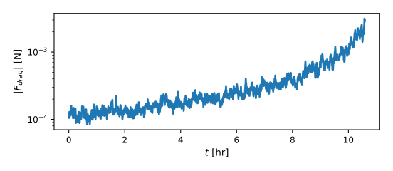
The magnitude of drag force over time:

scenarioStochasticDragSpacecraft.plotOrbits(timeAxis, posData, velData, dragForce, deterministicDenseData, oe, mu, planetRadius, dragCoeff, dragArea, figureTag='')

Plot orbit, altitude, atmosphere, correction, and drag.

figureTag is an optional tag inserted into figure names (e.g. “igbm”), so the variants get their own documentation images.

scenarioStochasticDragSpacecraft.run(showPlots: bool = False, rngSeed: int | None = None, useWind: bool = False, useIgbm: bool = False)

Run the spacecraft-based stochastic drag scenario.

Parameters:

• showPlots – If True, display figures.

• rngSeed – Optional stochastic integrator seed for reproducibility.

• useWind (bool) – If True, link a ZeroWindModel via SPICE so drag is computed against the atmosphere-relative velocity. If False (default), the inertial spacecraft velocity is used directly.

• useIgbm (bool) – If True, model the density correction factor with an inhomogeneous geometric Brownian motion (multiplicative noise, strictly positive factor) instead of the additive Ornstein-Uhlenbeck correction. Defaults to False.

Returns:

Dict of matplotlib figure handles.