scenarioGaussMarkovRandomWalk
Overview
This script demonstrates the difference between bounded Gauss-Markov random walk and pure Gaussian noise by simulating two IMU sensors with different configurations. The simulation shows how the Gauss-Markov process can be configured either to maintain bounded random walk behavior or to generate pure Gaussian noise. The script sets up a spacecraft in an elliptical Earth orbit and attaches two IMU sensors with different noise configurations.
The script is found in the folder basilisk/examples and executed by using:
python3 scenarioGaussMarkovRandomWalk.py
When the simulation completes a plot is shown for the IMU sensor measurements over time.
Simulation Scenario Setup Details
The simulation layout is shown in the following illustration. A single simulation process is created which contains both the spacecraft simulation module and two IMU sensor modules. Each IMU sensor has different configurations for the process noise (P Matrix), state propagation (A Matrix), and walk bounds.
The dynamics simulation is setup using a C++ Module: spacecraft module in an elliptical Earth orbit. The IMU sensors are configured with different parameters:
- IMU 1 demonstrates bounded random walk behavior:
Uses an identity A Matrix for state propagation
Has positive error bounds (±3.0 rad/s by default)
Shows random-walk behavior characteristic of an integrated process
Uses process noise level of 0.5 by default
- IMU 2 demonstrates pure Gaussian noise:
Uses the default zero A Matrix
Leaves hard clipping disabled
Shows independent noise samples with no temporal correlation
Uses the same process noise level as IMU 1
Both IMUs use the same process noise level (P Matrix) to ensure comparable noise magnitudes.
Setting only the IMU PMatrix produces white noise by default. This scenario
sets AMatrix and error bounds explicitly only for the bounded random-walk
sensor.
Illustration of Simulation Results
The following plot shows the angular velocity measurements from both IMU sensors over a 10-minute period:
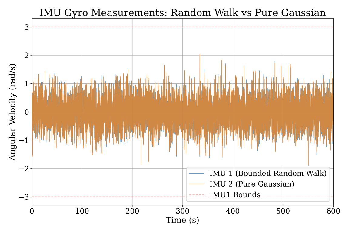
The plot demonstrates how: - IMU 1 (blue) exhibits bounded random walk behavior within ±3.0 rad/s bounds - IMU 2 (orange) shows pure Gaussian noise without temporal correlation - The bounded random walk maintains memory of previous states and shows smoother transitions - The pure Gaussian noise shows more rapid, independent variations
The simulation provides insight into how different Gauss-Markov process configurations affect sensor measurement behavior and demonstrates the flexibility of the model to generate both bounded random walk and pure Gaussian noise patterns.