scenarioOrbitFromOmm
Overview
Initialize two Basilisk spacecraft from an Orbit Mean-Elements Message (OMM)
file, then propagate them with point-mass Earth gravity. The bundled
dataForExamples/ommExample.kvn contains synthetic teaching data, not
observations or predictions for real satellites. One orbit is nearly circular
and inclined; the other is eccentric and near-polar. Both use fictitious
nine-digit catalog numbers and the same UTC epoch.
Run from the repository root with an installed Basilisk build:
python examples/scenarioOrbitFromOmm.py
The sample path is resolved relative to this script, so running from another
working directory also works. Keep dataForExamples/ommExample.kvn alongside
the script when copying the example. No network downloads, SPICE kernels,
gravity coefficient files, or Vizard installation are needed.
Read the file and inspect its metadata
Basilisk.utilities.ommHandling.satOmm2elem() detects KVN, XML, JSON,
or CSV from the file contents; the same call handles all four encodings:
from pathlib import Path
from Basilisk.utilities import ommHandling

path = Path(__file__).resolve().parent / "dataForExamples" / "ommExample.kvn"
records = ommHandling.satOmm2elem(str(path))
record = records[0]
print(record.satName, record.noradID, record.ommEpoch)
Catalog IDs are strings, preserving nine-digit IDs and leading zeros.
ommEpoch is a UTC datetime without a timezone object. meanMotion retains
the input mean motion in revolutions per day. The supported profile is
Earth-centered, TEME, UTC, and SGP4. The sample declares this profile and the
physical units explicitly. Malformed or unsupported records produce a warning
and are skipped, so check the returned list before selecting a satellite.
Unrecoverable file-level errors raise an exception.
Use the converted elements to initialize a spacecraft
OMM contains SGP4 mean elements. The reader initializes SGP4, evaluates the
state at the record epoch, converts TEME to the Basilisk inertial frame, and
derives osculating classical elements in record.oe. Use these elements
for initialization:
from Basilisk.utilities import orbitalMotion

r_N, v_N = orbitalMotion.elem2rv(earth.mu, record.oe)
vehicle.hub.r_CN_NInit = r_N  # [m]
vehicle.hub.v_CN_NInit = v_N  # [m/s]
Here earth is the Earth gravity body and vehicle is a Spacecraft, as
created in run(). The returned semi-major axis is in meters; inclination,
ascending node, argument of periapsis, and true anomaly are in radians.
Eccentricity is dimensionless. Do not apply another degrees-to-radians
conversion, interpret the input mean anomaly as true anomaly, or apply another
TEME rotation to record.oe.
Simulation time zero represents the common OMM epoch. This example rejects records with different epochs: a catalog’s states must first be propagated to a common epoch before they can describe simultaneous initial conditions. Static point-mass Earth gravity does not need a separate UTC clock or SPICE interface; models with time-dependent ephemerides would also need that setup.
Interpret the results
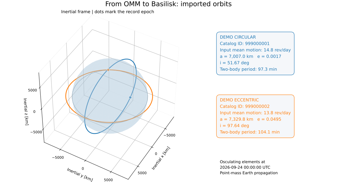
The first figure shows the orbital planes, initial positions, and imported osculating elements. The Earth sphere and the axes share the same length scale.
The second figure covers two periods of the slower spacecraft. The eccentric spacecraft moves fastest near perigee and slowest near apogee. Dashed altitude guides come from \(a(1-e)-R_E\) and \(a(1+e)-R_E\) using the imported osculating elements. Altitude here means distance from Earth’s center minus its equatorial radius, not height above an ellipsoid or terrain.
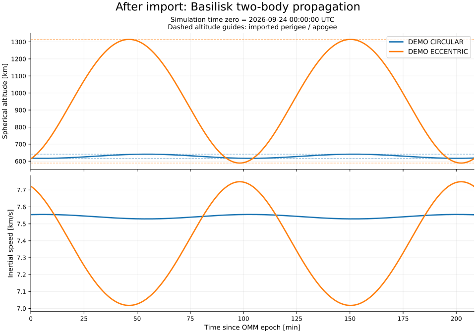
SGP4 supplies the initial state only. Subsequent motion in this example uses
Basilisk’s two-body dynamics, which omit Earth’s oblateness, atmospheric drag,
and other perturbations. The retained bStar, nDot, and nDotDot fields
do not configure Basilisk force models. These curves therefore illustrate the
handoff to a simulation, rather than continued SGP4 predictions or a validation
of the frame-conversion mathematics.
Try another file
From Python in the examples directory:
import scenarioOrbitFromOmm

results, figures = scenarioOrbitFromOmm.run(False, omm_path="my_catalog.json")
figures["scenarioOrbitFromOmmOrbits"].savefig("imported-orbits.svg")
Use records at a common epoch with bound orbits that remain above Earth.
results contains the epoch, gravitational parameter, reference Earth
radius, and each satellite’s imported record and sampled Cartesian states.
Figures remain available for saving when interactive display is disabled.
- scenarioOrbitFromOmm.run(show_plots, omm_path=None)[source]
Import a common-epoch catalog and simulate two periods of its slowest orbit.
- Parameters:
show_plots – whether to display the Matplotlib figures
omm_path – optional path to a KVN, XML, JSON, or CSV OMM file
- Returns:
results dictionary and a dictionary of named Matplotlib figures
- Raises:
ValueError – if no usable records remain, epochs differ, or an imported orbit is unbound or intersects the reference Earth sphere